An Introduction to 3D Reconstruction

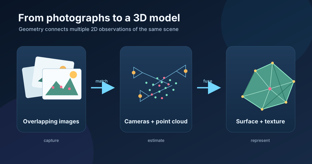
A photograph records how a three-dimensional scene looks from one position. 3D reconstruction tries to reverse that projection: given one or more observations, estimate the shape, position, and sometimes the appearance of the objects that produced them.

This problem appears in robotics, autonomous driving, surveying, visual effects, cultural heritage, e-commerce, and augmented reality. The required output differs by application. A robot may need an accurate occupancy map, a game artist may need an editable textured mesh, while a virtual-tour system may care most about rendering convincing new camera views.

This article develops a map of the field. We will cover:

What information is lost when a scene becomes an image.
The most common 3D representations.
The classical Structure-from-Motion and multi-view stereo pipeline.
Sensor-based, learning-based, and neural-rendering approaches.
How to choose an approach and evaluate its result.

Photographs are matched to estimate cameras and points, then fused into a textured surface

Defining the problem

Let a 3D point in world coordinates be

\mathbf{X} = [X, Y, Z, 1]^T.

A perspective camera maps it to an image point $\mathbf{x}$ :

s\mathbf{x} = \mathbf{K}[\mathbf{R}\mid\mathbf{t}]\mathbf{X}.

Here:

$\mathbf{K}$ contains the camera’s intrinsic parameters, such as focal length and principal point.
$\mathbf{R}$ and $\mathbf{t}$ describe the camera pose relative to the world.
$s$ is a depth-dependent scale factor.

Projection maps many possible 3D points onto the same pixel. A pixel identifies a ray, not a unique position along that ray. Reconstruction therefore needs another source of information: observations from another viewpoint, known camera motion, active depth sensing, physical constraints, or learned priors about likely scenes.

This leads to several related tasks:

Task	Typical input	Typical output
Monocular depth estimation	One RGB image	A depth value per pixel
Stereo reconstruction	A calibrated camera pair	Dense depth or disparity
Structure from Motion (SfM)	Multiple overlapping images	Camera poses and sparse 3D points
Multi-View Stereo (MVS)	Images with known cameras	Dense points or depth maps
SLAM	A live camera or depth stream	Camera trajectory and an evolving map
Novel-view synthesis	Images of a scene	Images rendered from new viewpoints

These tasks overlap, but they are not interchangeable. In particular, a representation that renders beautiful unseen views does not automatically provide an accurate, watertight surface.

Why reconstruction is difficult

The inverse problem is ill-posed: different scenes can explain the same images. Several ambiguities appear repeatedly.

Depth and scale

With a single uncalibrated image, absolute depth is not observable. A small nearby object can have the same projection as a large distant object. A moving monocular camera can often recover the scene only up to one global scale unless metric information is added.

Correspondence

Multi-view methods must determine which pixels observe the same physical point. Repeated windows, blank walls, changing illumination, motion blur, and large viewpoint changes make matching unreliable.

Occlusion and missing evidence

A camera sees only the first surface along each ray. The back of an object and regions hidden behind foreground geometry cannot be measured from that view. Any reconstruction of never-observed regions comes from assumptions or learned priors.

Non-Lambertian appearance

Classical stereo assumes that a surface patch has a similar appearance across views. Mirrors, glass, glossy materials, water, and exposure changes violate this assumption. Their highlights move with the camera and can be mistaken for geometry.

Dynamic scenes

Most pipelines assume a static world. People, vehicles, foliage, and rolling-shutter effects break the geometric consistency between frames. A method must reject these observations or model time and deformation explicitly.

Choosing a 3D representation

“A 3D model” can refer to very different data structures:

Representation	Strengths	Limitations
Depth map	Dense, image-aligned, easy to predict	Describes one viewpoint; does not join surfaces
Point cloud	Simple, preserves measured samples	No explicit surface; holes and noise are visible
Voxel grid	Easy occupancy queries and 3D convolutions	Memory grows cubically with resolution
Mesh	Compact surface, editable, supported by graphics tools	Topology and hole filling can be difficult
Signed distance field (SDF)	Continuous surface and meaningful inside/outside test	Must be sampled or converted for rendering
Radiance field	Excellent view-dependent appearance and novel views	Geometry can be indirect or ambiguous
3D Gaussians	Fast differentiable rendering and explicit primitives	Not inherently a clean, watertight surface

The right representation follows the downstream goal. Collision checking favors occupancy or signed distance; manufacturing requires metric surfaces; web viewing favors compact meshes; photorealistic replay favors radiance fields or Gaussian splats.

Approach 1: classical multi-view geometry

The classical image-based pipeline separates reconstruction into interpretable geometric stages. Its two major components are Structure from Motion, which recovers cameras and sparse structure, and Multi-View Stereo, which densifies that structure.

1. Detect and match features

The pipeline finds distinctive keypoints in each image and describes their local appearance. It then proposes matches between images. Geometric verification, commonly with RANSAC and epipolar constraints, rejects many incorrect matches.

Good image overlap matters more than raw image count. If consecutive views share too little content, the matching graph becomes disconnected. If views are almost identical, triangulation has too little baseline to estimate depth accurately.

2. Estimate camera poses

Matched points constrain the relative motion between cameras. An incremental SfM system initializes from a reliable image pair, triangulates points, registers more cameras, and repeats. The result is a sparse point cloud and a pose for every registered image.

The open-source COLMAP pipeline is based on this family of methods. Its SfM design is described in Structure-from-Motion Revisited.

3. Refine with bundle adjustment

Initial camera poses and 3D points contain error. Bundle adjustment jointly refines both by minimizing reprojection error:

\min_{\{\mathbf{P}_i\},\{\mathbf{X}_j\}} \sum_{(i,j)\in\mathcal{V}} \rho\left( \left\| \mathbf{x}_{ij} - \pi(\mathbf{P}_i,\mathbf{X}_j) \right\|_2^2 \right).

$\mathbf{x}_{ij}$ is the observed location of point $j$ in image $i$ , $\pi$ is the camera projection function, $\mathcal{V}$ contains visible point-camera pairs, and $\rho$ is a robust loss that reduces the influence of outliers.

Bundle adjustment is one of the central ideas in multi-view geometry: a reconstruction should explain all observations consistently, not just each image pair in isolation.

4. Recover dense geometry

Sparse feature points are sufficient for pose estimation but not for a complete model. MVS searches for correspondence at many more pixels, estimates a depth map for each view, checks agreement across views, and fuses consistent samples into a dense cloud.

Traditional MVS uses hand-designed photometric costs and regularization. Learned methods such as MVSNet replace parts of this stage with learned image features and a 3D cost volume, while retaining explicit multi-view warping.

5. Build and texture a surface

The dense point cloud can be filtered, converted to a mesh, simplified, and textured from the source photographs. This stage must balance detail against noise. Aggressive smoothing removes artifacts but can also erase thin structures and sharp edges.

When classical geometry works well

This approach remains a strong choice when:

The scene is static and has textured, mostly diffuse surfaces.
Images have reliable overlap, focus, and exposure.
Camera calibration is known or can be estimated.
Metric geometry and inspectable failure modes matter.

Its weaknesses are equally predictable: textureless regions produce holes, reflections create false matches, and a poor capture path can prevent pose recovery entirely.

Approach 2: active depth and range sensing

Instead of inferring depth only from passive RGB images, a system can measure it more directly.

Structured light projects a known pattern and estimates how the pattern deforms.
Time-of-Flight (ToF) measures the travel time or phase shift of emitted light.
LiDAR scans laser returns to produce metric ranges.
RGB-D cameras align a depth sensor with a color camera.

Successive depth frames are transformed into a common coordinate system and fused, often into a voxel occupancy map or truncated signed distance field (TSDF). Camera tracking may use RGB features, depth alignment, inertial measurements, or a combination.

Sensor-based reconstruction offers metric scale and can work on surfaces with little visual texture. The tradeoffs are hardware cost, limited range or resolution, multipath interference, sunlight sensitivity, and missing returns from transparent or highly reflective materials.

Approach 3: learning-based depth and geometry

Neural networks can learn priors that classical matching does not have. A model may recognize that floors are usually planar, cars have a typical shape, and object boundaries often coincide with depth discontinuities.

Single-view depth

A monocular model predicts depth from one image. Because geometry alone cannot resolve the ambiguity, the prediction depends heavily on patterns learned from training data. It can be useful for scene understanding and as an initialization, but its scale may be unknown and unfamiliar scenes can produce plausible yet incorrect geometry.

This distinction is important: prediction is not measurement. A network can complete an unseen surface because similar surfaces appeared in its training data, not because the input image contained evidence for that surface.

Learned stereo and multi-view reconstruction

Learned stereo methods still use multiple views, but compare learned features rather than raw colors and use a network to regularize ambiguous matches. Cost-volume approaches evaluate candidate depths by warping source-view features into a reference camera. They often handle weak texture better than purely hand-crafted matching, though memory usage grows with image size and the sampled depth range.

Feed-forward 3D models

A newer family of models predicts several geometric quantities directly from images. DUSt3R regresses pairwise point maps and aligns them in a shared frame, reducing the need for known calibration and camera poses. VGGT predicts camera parameters, depth maps, point maps, and point tracks in one feed-forward model.

These systems make unconstrained image collections easier to process and can provide strong initialization. They also introduce learned failure modes, domain dependence, high model cost, and less transparent uncertainty. For measurement-critical work, their output should still be checked against calibrated geometry or ground truth.

Approach 4: neural radiance fields

A Neural Radiance Field, or NeRF, represents a scene as a continuous function. The original formulation maps a 3D position $\mathbf{x}$ and viewing direction $\mathbf{d}$ to volume density $\sigma$ and color $\mathbf{c}$ :

F_\theta(\mathbf{x}, \mathbf{d}) \rightarrow (\sigma, \mathbf{c}).

For each camera ray, the renderer samples this function and integrates color through the volume. Because rendering is differentiable, the parameters can be optimized so that rendered views reproduce the input photographs.

The original NeRF paper demonstrated high-quality novel-view synthesis from images with known camera poses. Later systems improved training speed, scene scale, relighting, dynamic content, and surface extraction.

NeRF is best understood first as a view-synthesis representation. Density often correlates with surfaces, and meshes can be extracted, but photometric optimization may place semi-transparent density in geometrically incorrect locations. If accurate geometry is the goal, the method should include geometric regularization or depth supervision and be evaluated as geometry, not only by rendered image quality.

Approach 5: 3D Gaussian splatting

3D Gaussian Splatting (3DGS) represents a scene with many anisotropic Gaussian primitives. Each Gaussian has a position, orientation, scale, opacity, and appearance parameters. During rendering, the primitives are projected onto the image, ordered by depth, and alpha-composited.

The original 3D Gaussian Splatting paper initializes from sparse SfM points and jointly optimizes the primitives against input views. Its rasterization-based renderer makes interactive novel-view rendering practical.

Compared with a basic NeRF:

The scene is stored as explicit primitives instead of only in network weights.
Rendering is generally faster because empty space does not need dense ray sampling.
Editing and spatial inspection are more direct.
The optimized Gaussians still do not form a conventional surface.

3DGS is a strong choice for photorealistic scene replay, but converting splats into a clean mesh remains a separate reconstruction problem.

Approach 6: generative single-image reconstruction

Generative models can infer a 3D object or synthesize additional views from a single photograph, then reconstruct from those views. This is attractive for asset creation because capture is minimal.

The fundamental limitation does not disappear: the input contains no observation of the hidden side. The model produces a statistically plausible completion, not a uniquely recovered object. That may be acceptable for entertainment or rapid prototyping, but it is unsuitable when hidden geometry must match a real artifact.

It helps to reserve the word reconstruction for observed evidence and use completion or generation for inferred, unobserved content.

Comparing the main approaches

Approach	Main input	Best at	Main weakness
SfM + MVS	Many overlapping RGB images	Accurate, inspectable geometry	Sensitive to capture quality and material
Active depth / LiDAR	Range measurements, often RGB	Metric scale and low-texture surfaces	Hardware and sensor-specific artifacts
Learned depth / MVS	One or more images	Fast inference and learned priors	Domain shift and geometric hallucination
Feed-forward 3D models	Uncalibrated image collections	Rapid cameras, depth, and point maps	Compute cost and learned failure modes
NeRF	Posed images	Smooth photorealistic novel views	Training cost and indirect geometry
3D Gaussian Splatting	Posed images, often SfM points	Fast high-quality view synthesis	No inherent watertight surface
Generative 3D	One or a few images	Plausible asset creation	Unseen geometry is invented

Hybrid systems are common. SfM may estimate cameras for NeRF or 3DGS; a depth network may initialize MVS; LiDAR may anchor a radiance field to metric scale; and neural rendering may add appearance to a mesh-based scan.

Evaluating a reconstruction

There is no single score for every output. Choose metrics that reflect the intended use.

Geometry metrics

Given predicted point set $P$ and reference point set $G$ , a symmetric Chamfer distance is:

d_{\mathrm{CD}}(P,G) = \frac{1}{|P|}\sum_{p\in P}\min_{g\in G}\|p-g\|_2^2 + \frac{1}{|G|}\sum_{g\in G}\min_{p\in P}\|g-p\|_2^2.

It measures proximity in both directions, but averages can hide local defects. Common complementary measures include:

Accuracy: how close predicted points are to the reference.
Completeness: how much of the reference surface was recovered.
Precision, recall, and F-score at a distance threshold.
Normal consistency for surface orientation.
Absolute trajectory error for camera tracking.

Metric evaluation requires aligned coordinate systems. If a monocular reconstruction has unknown scale, similarity alignment can make shape comparisons fair, but the result should not be described as metric accuracy.

Rendering metrics

Novel-view systems are often evaluated on held-out images using:

PSNR for pixel-level reconstruction error.
SSIM for structural similarity.
LPIPS for perceptual feature similarity.

High rendering scores do not prove that the underlying geometry is correct. A rigorous evaluation reports geometry and appearance separately whenever both matter.

Operational qualities

Production systems also care about capture time, reconstruction latency, memory, render speed, robustness, model size, editability, and export compatibility. A slightly less accurate mesh that opens reliably in standard tools may be more useful than a visually impressive representation tied to one renderer.

A practical capture checklist

For an image-based reconstruction:

Decide the output first. A measurement mesh, a virtual tour, and a game asset need different pipelines.
Keep the scene static. Remove moving objects where possible.
Capture consistent overlap. Aim for roughly 60–80% overlap between neighboring views.
Move around the subject. Translation creates parallax; rotating from one position does not provide the same depth evidence.
Lock focus and exposure. Avoid blur, large exposure jumps, and digital zoom.
Include texture where possible. Temporary markers can help on blank surfaces, if the application permits them.
Cover every required surface. The algorithm cannot measure a region that no camera or sensor observed.
Hold out a few views. Use them to test rendering quality instead of optimizing and evaluating on the same images.
Inspect intermediate results. Check image matches, camera poses, sparse points, depth maps, and only then the final mesh or renderer.

Which approach should you start with?

For an accurate object or site model from photographs, start with calibrated capture and an SfM + MVS pipeline.
For indoor mapping or robotics, use RGB-D, LiDAR, or visual-inertial SLAM when hardware permits.
For photorealistic novel views, begin with 3DGS when fast rendering matters, or a NeRF-family method when its continuous representation better fits the task.
For fast geometry from casual, uncalibrated photos, test feed-forward models, then refine or validate their output geometrically.
For one-image asset creation, use generative reconstruction only when plausible hidden geometry is sufficient.

The central engineering decision is not “Which method is newest?” It is “Which parts of the scene must be measured, which may be inferred, and what will the result be used for?”

Conclusion

3D reconstruction is a family of inverse problems rather than one algorithm. Classical methods recover geometry by enforcing agreement across calibrated views. Depth sensors measure range directly. Learned models contribute powerful priors. NeRF and 3D Gaussian Splatting optimize scene representations for rendering, while generative methods fill gaps with plausible content.

All of them trade among accuracy, completeness, capture effort, compute, and visual quality. Once the input evidence, output representation, and evaluation criteria are explicit, choosing a pipeline becomes much more straightforward.

An Introduction to 3D Reconstruction: From Images to Geometry