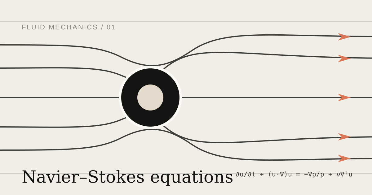
Why these equations matter

The Navier–Stokes equations describe how the velocity, pressure, density, and temperature of a fluid evolve. They sit behind weather prediction, aircraft design, blood-flow simulation, ocean circulation, combustion, and the movement of water through a pipe. Their ingredients are familiar—Newton’s second law, conservation of mass, and a constitutive model for viscous stress—but their nonlinear interaction can produce vortices, boundary layers, and turbulence across an enormous range of scales.

This article focuses on the incompressible, constant-property equations. That model is appropriate when density variations are negligible, as in many flows of water and low-speed air. Compressible flow additionally couples momentum to mass, energy, and an equation of state.

The fields and assumptions

At every position $\mathbf{x}$ and time $t$, we seek:

• the velocity field $\mathbf{u}(\mathbf{x},t)$, measured in $\mathrm{m\,s^{-1}}$;
• the pressure field $p(\mathbf{x},t)$, measured in $\mathrm{Pa}$;
• the density $\rho$, measured in $\mathrm{kg\,m^{-3}}$;
• the dynamic viscosity $\mu$, measured in $\mathrm{Pa\,s}$.

The kinematic viscosity is $\nu=\mu/\rho$, with units $\mathrm{m^2\,s^{-1}}$. We treat the fluid as a continuum: each computational point represents an average over many molecules, so differentiable fields are meaningful.

The material derivative follows a moving fluid parcel:

$$\frac{D}{Dt}=\frac{\partial}{\partial t}+\mathbf{u}\cdot\nabla.$$

It combines local change at a fixed point with change caused by transport through a spatial gradient.

Conservation of mass

For a compressible fluid, local mass conservation gives the continuity equation:

$$\frac{\partial \rho}{\partial t}+\nabla\cdot(\rho\mathbf{u})=0.$$

If density is constant, this reduces to the incompressibility constraint:

$$\boxed{\nabla\cdot\mathbf{u}=0.}$$

This does not say that the velocity is constant. It says that a small material volume does not expand or contract. Whatever fluid enters a control volume must leave it at the same rate.

Conservation of momentum

Newton’s second law for a continuum states that mass times acceleration equals surface and body forces:

$$\rho\frac{D\mathbf{u}}{Dt}=\nabla\cdot\boldsymbol{\sigma}+\rho\mathbf{f},$$

where $\boldsymbol{\sigma}$ is the Cauchy stress tensor and $\mathbf{f}$ is a body force per unit mass, such as gravity. Split stress into pressure and viscous parts:

$$\boldsymbol{\sigma}=-p\mathbf{I}+\boldsymbol{\tau}.$$

For a Newtonian fluid,

$$\boldsymbol{\tau} =\mu\left(\nabla\mathbf{u}+(\nabla\mathbf{u})^T\right) +\lambda(\nabla\cdot\mathbf{u})\mathbf{I}.$$

With constant $\rho$ and $\mu$, and with $\nabla\cdot\mathbf{u}=0$, the system becomes

$$\boxed{ \frac{\partial\mathbf{u}}{\partial t} +(\mathbf{u}\cdot\nabla)\mathbf{u} =-\frac{1}{\rho}\nabla p +\nu\nabla^2\mathbf{u} +\mathbf{f}, \qquad \nabla\cdot\mathbf{u}=0. }$$

Reading the momentum equation term by term

Term	Meaning
$\partial\mathbf{u}/\partial t$	Local acceleration at a fixed point
$(\mathbf{u}\cdot\nabla)\mathbf{u}$	Convective acceleration; velocity transports itself
$-\nabla p/\rho$	Acceleration caused by pressure differences
$\nu\nabla^2\mathbf{u}$	Viscous diffusion of momentum
$\mathbf{f}$	Body forcing per unit mass

The convection term is nonlinear because the unknown velocity multiplies its own gradient. Pressure has a special role in incompressible flow: it adjusts so that the updated velocity remains divergence-free. Mathematically, it behaves like a Lagrange multiplier enforcing $\nabla\cdot\mathbf{u}=0$.

Dimensionless form and the Reynolds number

Choose a characteristic length $L$ and speed $U$, then define

$$\mathbf{x}=L\mathbf{x}^*,\qquad t=\frac{L}{U}t^*,\qquad \mathbf{u}=U\mathbf{u}^*,\qquad p=\rho U^2p^*.$$

After substitution and removal of the stars, the unforced equation is

$$\frac{\partial\mathbf{u}}{\partial t} +(\mathbf{u}\cdot\nabla)\mathbf{u} =-\nabla p+\frac{1}{\mathrm{Re}}\nabla^2\mathbf{u},$$

where

$$\boxed{\mathrm{Re}=\frac{\rho UL}{\mu}=\frac{UL}{\nu}.}$$

The Reynolds number compares inertial transport with viscous diffusion. Low-$\mathrm{Re}$ flows are usually smooth and strongly damped; high-$\mathrm{Re}$ flows can develop thin shear layers, instabilities, and turbulence. Reynolds number alone does not determine a flow—the geometry, forcing, and boundary conditions also matter—but it is the first similarity parameter to inspect.

Initial and boundary conditions

A differential equation is not a complete flow problem until its domain and data are specified.

• Initial condition: prescribe a divergence-free velocity $\mathbf{u}(\mathbf{x},0)=\mathbf{u}_0(\mathbf{x})$.
• No-slip wall: set fluid velocity equal to wall velocity. A stationary wall has $\mathbf{u}=0$.
• Inflow: prescribe a compatible velocity profile or mass flow rate.
• Outflow: often prescribe pressure and use a weak condition for velocity, while keeping the boundary far from recirculation.
• Periodic boundary: match fields across paired faces, useful for idealized channels and homogeneous turbulence.
• Free-slip or symmetry boundary: prevent normal flow while setting tangential shear to zero.

Boundary conditions for pressure are coupled to the velocity conditions; assigning both arbitrarily can overconstrain the system.

Two exact flows that build intuition

Couette flow

Place fluid between parallel plates at $y=0$ and $y=h$. Keep the lower plate fixed and move the upper plate at speed $U$. For steady, fully developed flow with no pressure gradient, $\mathbf{u}=(u(y),0,0)$ and

$$\mu\frac{d^2u}{dy^2}=0.$$

Applying $u(0)=0$ and $u(h)=U$ gives

$$\boxed{u(y)=U\frac{y}{h}.}$$

Viscosity communicates the moving wall’s momentum through the fluid, producing a linear profile and constant shear stress $\tau_{xy}=\mu U/h$.

Plane Poiseuille flow

Now keep both plates fixed at $y=\pm h$ and drive the flow with a constant pressure gradient $dp/dx<0$. The equation reduces to

$$0=-\frac{dp}{dx}+\mu\frac{d^2u}{dy^2}.$$

With $u(-h)=u(h)=0$,

$$\boxed{ u(y)=-\frac{1}{2\mu}\frac{dp}{dx}(h^2-y^2). }$$

The profile is parabolic. Its maximum occurs at the centerline, and its cross-sectional mean is $\bar{u}=\tfrac{2}{3}u_{\max}$ for this plane channel.

Vorticity and kinetic energy

Vorticity measures local rotation:

$$\boldsymbol{\omega}=\nabla\times\mathbf{u}.$$

Taking the curl of the incompressible momentum equation yields

$$\frac{\partial\boldsymbol{\omega}}{\partial t} +(\mathbf{u}\cdot\nabla)\boldsymbol{\omega} =(\boldsymbol{\omega}\cdot\nabla)\mathbf{u} +\nu\nabla^2\boldsymbol{\omega} +\nabla\times\mathbf{f}.$$

The term $(\boldsymbol{\omega}\cdot\nabla)\mathbf{u}$ stretches and tilts vortices in three dimensions. It vanishes for strictly two-dimensional incompressible flow, one reason the mathematical behavior of the 2D equations is better controlled.

Under periodic boundaries or suitable decay/no-slip conditions, the kinetic-energy balance is

$$\frac{1}{2}\frac{d}{dt}\int_\Omega |\mathbf{u}|^2\,d\mathbf{x} =-\nu\int_\Omega |\nabla\mathbf{u}|^2\,d\mathbf{x} +\int_\Omega \mathbf{f}\cdot\mathbf{u}\,d\mathbf{x}.$$

Convection and pressure redistribute energy; viscosity removes it. This identity is both physical insight and a valuable check for numerical solvers.

How a projection method solves the equations

Most realistic geometries require numerical approximation. Finite differences, finite volumes, finite elements, and spectral methods discretize space differently, but every incompressible solver must couple velocity and pressure while maintaining near-zero divergence.

A basic projection method advances one time step in three stages. First, predict a velocity without the new pressure:

$$\mathbf{u}^*=\mathbf{u}^n+\Delta t\left[ -(\mathbf{u}^n\cdot\nabla)\mathbf{u}^n +\nu\nabla^2\mathbf{u}^n+\mathbf{f}^n \right].$$

Next, solve a pressure Poisson equation:

$$\nabla^2p^{n+1}=\frac{\rho}{\Delta t}\nabla\cdot\mathbf{u}^*.$$

Finally, project the velocity onto the divergence-free space:

$$\mathbf{u}^{n+1}=\mathbf{u}^*-\frac{\Delta t}{\rho}\nabla p^{n+1}.$$

The algorithmic skeleton is compact:

for step in range(num_steps):
    convection = advect(velocity)
    diffusion = viscosity * laplacian(velocity)
    predicted = velocity + dt * (-convection + diffusion + force)

    rhs = density / dt * divergence(predicted)
    pressure = solve_poisson(rhs, pressure_boundary_conditions)

    velocity = predicted - dt / density * gradient(pressure)
    velocity = apply_velocity_boundary_conditions(velocity)

A production solver must also use consistent discrete gradient/divergence operators, stable advection, appropriate linear solvers, mesh-quality checks, and pressure boundary conditions. For explicit schemes, useful scale estimates are

$$\Delta t\lesssim C\frac{\Delta x}{U_{\max}}, \qquad \Delta t\lesssim C_\nu\frac{\Delta x^2}{\nu},$$

for convective and diffusive stability, respectively. The constants depend on dimension and discretization.

The existence and smoothness problem

In two dimensions, sufficiently regular incompressible data lead to global smooth solutions. In three dimensions, global Leray weak solutions exist, but their uniqueness and full regularity are unknown. The open question is whether every smooth, finite-energy, divergence-free initial condition produces a solution that remains smooth for all time, or whether a singularity can form in finite time.

This is one of the Clay Mathematics Institute’s Millennium Prize Problems. A turbulent computation with extremely small scales is not evidence of a mathematical singularity: numerical resolution, discretization error, and the distinction between weak and classical solutions all matter.

A practical checklist

When formulating or reviewing an incompressible-flow model, ask:

1. Is constant density justified, or is a compressible/variable-density model required?
2. What are the characteristic $U$, $L$, and Reynolds number?
3. Are initial and boundary data mutually compatible and mass-conserving?
4. Does the mesh resolve walls, shear layers, and relevant turbulent scales?
5. Is the time step consistent with convective and diffusive stability limits?
6. Does the discrete velocity remain divergence-free?
7. Do mass, momentum, and energy budgets close to the expected tolerance?
8. Has the result been checked against an exact solution, benchmark, or grid-refinement study?

The equations are compact; trustworthy solutions are not. Good fluid mechanics comes from combining the conservation laws with careful modeling, boundary conditions, numerics, and validation.

Further reading

• Clay Mathematics Institute: Navier–Stokes Equation and the official problem description.
• NASA Glenn: Navier–Stokes Equations for the conservation-law form used in aerodynamics.
• A. J. Chorin, Numerical Solution of the Navier–Stokes Equations, for the projection-method idea.