Introduction

Most machine learning models learn from labeled examples. Reinforcement learning is different: an agent interacts with an environment, observes the consequences of its actions, and learns which decisions produce the largest long-term reward.

In this tutorial, we will implement Q-learning from scratch in Python. Our agent will learn to move through a small grid, avoid a trap and a wall, and reach a goal. The program uses only Python’s standard library, so the algorithm remains visible instead of being hidden behind a framework.

By the end, you will understand:

The states, actions, rewards, and episodes used in reinforcement learning.
The Q-learning update rule.
How epsilon-greedy exploration works.
How to train and evaluate a simple agent in Python.

The problem: navigate a grid world

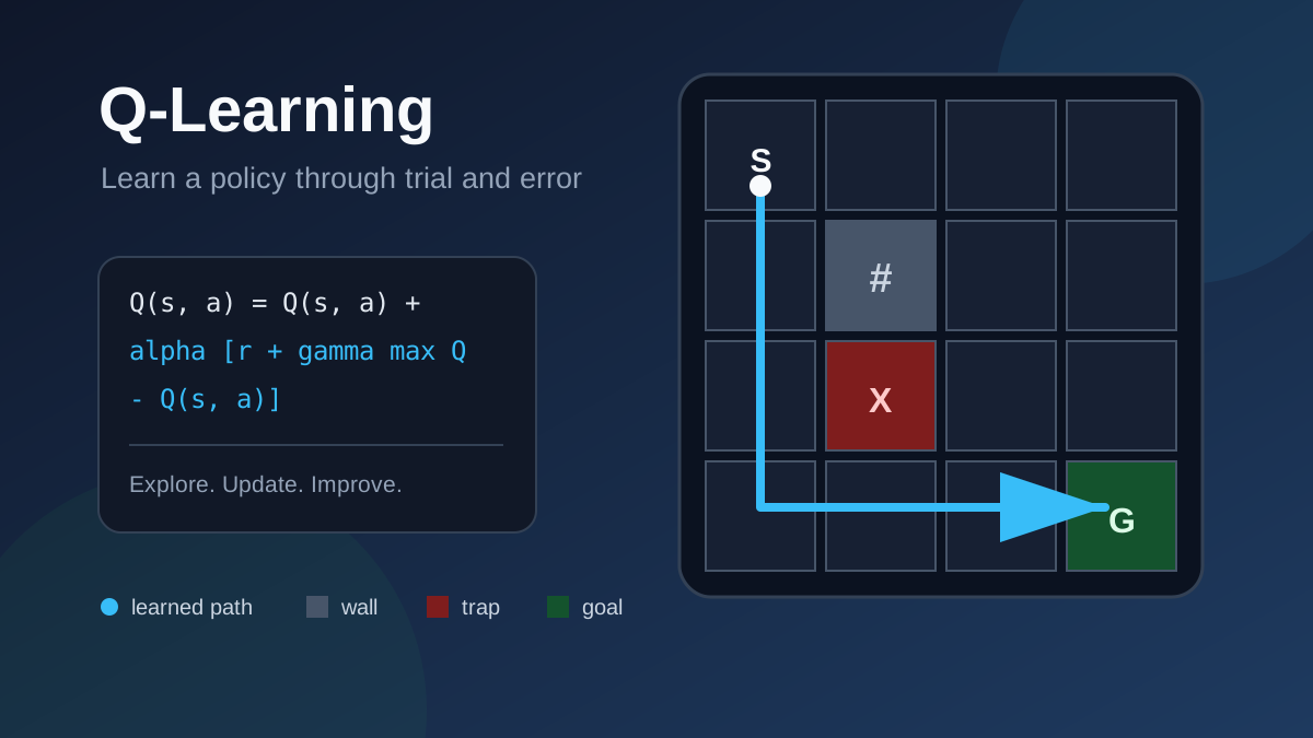
Consider this 4 x 4 environment:

S . . .
. # . .
. X . .
. . . G

S is the starting position.
G is the goal.
# is a wall that the agent cannot enter.
X is a trap that ends the episode.
. is an ordinary empty cell.

At every step, the agent can move up, down, left, or right. Moving outside the grid or into the wall leaves it in the same position.

We define the rewards as follows:

Event	Reward
Reach the goal	`+20`
Enter the trap	`-10`
Take a normal step	`-1`

The -1 step cost matters. Without it, the agent would have little reason to prefer a short path over a long one.

What is Q-learning?

Q-learning is a model-free, off-policy reinforcement-learning algorithm.

Model-free means the agent does not need to know the environment’s transition probabilities in advance. It learns by interacting with the environment.
Off-policy means the agent can explore using one behavior, such as random actions, while learning the value of a different behavior: always choosing the best known action.

The algorithm learns a function called the action-value function:

Q(s, a)

This value estimates the total discounted reward the agent can obtain by taking action $a$ in state $s$ , then behaving optimally afterward.

In a small environment, we can store these estimates in a table. Our grid contains 16 states and 4 actions, so the Q-table has $16 \times 4 = 64$ values:

State	Up	Down	Left	Right
`(0, 0)`	0.0	0.0	0.0	0.0
`(0, 1)`	0.0	0.0	0.0	0.0
…	…	…	…	…

All entries begin at zero. They improve as the agent collects experience.

The Q-learning update

After taking an action, the agent observes a transition:

(s, a, r, s')

Here, $s$ is the current state, $a$ is the selected action, $r$ is the reward, and $s'$ is the next state. Q-learning updates the selected table entry with:

Q(s,a) \leftarrow Q(s,a) + \alpha \left[ r + \gamma \max_{a'} Q(s',a') - Q(s,a) \right].

The terms are:

$\alpha$ , the learning rate, controls how strongly new information replaces an old estimate.
$\gamma$ , the discount factor, controls how much future rewards matter.
$\max_{a'} Q(s',a')$ is the best estimated value available from the next state.
The expression inside the brackets is the temporal-difference error.

For a terminal state, there is no future reward to estimate, so the next-state value is zero.

Exploration versus exploitation

If the agent always selects the action with the largest current Q-value, it may commit too early to a poor route. It needs to explore.

We will use an epsilon-greedy policy:

With probability $\epsilon$ , select a random action.
Otherwise, select an action with the highest Q-value.

Training begins with $\epsilon = 1.0$ , meaning the agent explores heavily. After each episode, epsilon decays until it reaches 0.05. The agent therefore becomes more consistent while retaining a small amount of exploration.

Implementing the environment

Create the grid constants and action definitions:

import random


ROWS, COLS = 4, 4
START = (0, 0)
GOAL = (3, 3)
WALLS = {(1, 1)}
TRAPS = {(2, 1)}

# up, down, left, right
ACTIONS = [(-1, 0), (1, 0), (0, -1), (0, 1)]
ACTION_NAMES = ["up", "down", "left", "right"]

A position such as (2, 3) is easy for people to read, but a list-based Q-table needs an integer index. We convert each position into a state ID:

def state_id(position):
    row, col = position
    return row * COLS + col

For example, (0, 0) becomes state 0, (0, 1) becomes state 1, and (3, 3) becomes state 15.

The step function contains the environment rules:

def step(position, action):
    """Apply an action and return (next_position, reward, done)."""
    row, col = position
    d_row, d_col = ACTIONS[action]
    candidate = (row + d_row, col + d_col)

    if not (0 <= candidate[0] < ROWS and 0 <= candidate[1] < COLS):
        candidate = position
    if candidate in WALLS:
        candidate = position

    if candidate == GOAL:
        return candidate, 20, True
    if candidate in TRAPS:
        return candidate, -10, True
    return candidate, -1, False

The returned done flag tells the training loop that the episode has ended.

Training the agent

When several actions share the highest value, choosing the first one every time introduces a fixed directional bias. This helper randomly breaks ties:

def argmax(values):
    """Return a random index among the maximum values."""
    best_value = max(values)
    best_actions = [
        index for index, value in enumerate(values)
        if value == best_value
    ]
    return random.choice(best_actions)

Now implement the training loop:

def train(
    episodes=3000,
    alpha=0.1,
    gamma=0.95,
    epsilon=1.0,
    epsilon_decay=0.995,
    epsilon_min=0.05,
):
    q_table = [
        [0.0 for _ in ACTIONS]
        for _ in range(ROWS * COLS)
    ]
    rewards = []

    for _ in range(episodes):
        position = START
        total_reward = 0

        for _ in range(100):
            state = state_id(position)

            if random.random() < epsilon:
                action = random.randrange(len(ACTIONS))
            else:
                action = argmax(q_table[state])

            next_position, reward, done = step(position, action)
            next_state = state_id(next_position)

            next_best = 0 if done else max(q_table[next_state])
            td_target = reward + gamma * next_best
            td_error = td_target - q_table[state][action]
            q_table[state][action] += alpha * td_error

            position = next_position
            total_reward += reward

            if done:
                break

        epsilon = max(epsilon_min, epsilon * epsilon_decay)
        rewards.append(total_reward)

    return q_table, rewards

Each episode starts at START. The agent selects actions, receives rewards, and updates one Q-value after every transition. The 100-step limit prevents a poorly trained agent from wandering forever.

The most important lines directly implement the Q-learning equation:

next_best = 0 if done else max(q_table[next_state])
td_target = reward + gamma * next_best
td_error = td_target - q_table[state][action]
q_table[state][action] += alpha * td_error

Inspecting the learned policy

A policy maps each state to an action. After training, we can derive a greedy policy by selecting the largest Q-value in every state:

def print_policy(q_table):
    arrows = ["^", "v", "<", ">"]

    for row in range(ROWS):
        cells = []

        for col in range(COLS):
            position = (row, col)

            if position == GOAL:
                cells.append("G")
            elif position in WALLS:
                cells.append("#")
            elif position in TRAPS:
                cells.append("X")
            else:
                state = state_id(position)
                action = max(
                    range(len(ACTIONS)),
                    key=lambda index: q_table[state][index],
                )
                cells.append(arrows[action])

        print(" ".join(cells))

We can also follow the greedy policy from the starting position:

def greedy_path(q_table, max_steps=20):
    position = START
    path = [position]

    for _ in range(max_steps):
        state = state_id(position)
        action = max(
            range(len(ACTIONS)),
            key=lambda index: q_table[state][index],
        )
        position, _, done = step(position, action)
        path.append(position)

        if done:
            break

    return path

Finally, train and evaluate the agent:

if __name__ == "__main__":
    random.seed(7)
    q_table, rewards = train()

    average_reward = sum(rewards[-100:]) / 100
    print(
        "Average reward over the final 100 episodes:",
        round(average_reward, 2),
    )
    print("Learned policy:")
    print_policy(q_table)
    print("Greedy path:", greedy_path(q_table))

The fixed random seed makes this tutorial reproducible. Run the complete program with:

python3 assets/misc_code/q_learning_grid_world.py

A typical result is:

Average reward over the final 100 episodes: 14.27
Learned policy:
v > v v
v # > v
v X v v
> > > G
Greedy path: [(0, 0), (1, 0), (2, 0), (3, 0),
              (3, 1), (3, 2), (3, 3)]

The greedy path takes six moves. It travels down the left edge and then across the bottom row, avoiding both the wall and the trap. Its undiscounted return is:

5(-1) + 20 = 15.

The final-100-episode average can be lower than 15 because training deliberately keeps a 5% exploration rate. Evaluation with the greedy policy disables that random exploration.

Understanding the hyperparameters

The defaults work well for this small deterministic problem, but each parameter has a distinct role:

Parameter	Value	Effect
`episodes`	`3000`	Number of training attempts
`alpha`	`0.1`	Speed of Q-value updates
`gamma`	`0.95`	Importance of future rewards
`epsilon`	`1.0`	Initial exploration probability
`epsilon_decay`	`0.995`	Exploration reduction per episode
`epsilon_min`	`0.05`	Minimum exploration probability

If learning is unstable, reduce alpha. If the agent ignores delayed rewards, increase gamma. If it settles on a bad route too quickly, decay epsilon more slowly.

Experiments to try

The fastest way to understand Q-learning is to change the environment and predict what should happen:

Move the trap to (3, 1) and observe the new route.
Change the normal step reward from -1 to 0. Does the agent still prefer the shortest path?
Increase the trap penalty to -100.
Add a second goal with a smaller reward.
Make actions stochastic, so the requested direction occasionally moves the agent elsewhere.

These experiments expose an important lesson: the agent optimizes the reward function you define, not necessarily the behavior you intended.

Limitations of tabular Q-learning

A Q-table works when the state and action spaces are small and discrete. It becomes impractical for images, continuous sensor values, or games with enormous numbers of states.

Common extensions include:

Deep Q-Networks (DQN), which replace the table with a neural network.
Double DQN, which reduces overestimation bias.
Policy-gradient methods, which learn a policy directly.
Actor-critic methods, which learn both a policy and a value estimate.

Despite those limitations, tabular Q-learning is an excellent starting point. It makes the central reinforcement-learning loop concrete: observe a state, choose an action, receive a reward, update an estimate, and repeat until useful behavior emerges.

Conclusion

Q-learning does not require examples of the correct action. Instead, it learns action values from trial and error and turns those values into a policy.

Our Python agent began with no knowledge of the grid. After repeated episodes, it learned a short path to the goal while avoiding the trap. The same ideas behind this 64-value table also appear in larger reinforcement-learning systems: temporal-difference updates, discounted rewards, and a deliberate balance between exploration and exploitation.