Linear Regression: Foundations, Estimation, and Diagnostics

Linear regression is a fundamental method for modeling the relationship between a continuous response variable and one or more explanatory variables. It is widely used for prediction, estimation, hypothesis testing, and the analysis of relationships between variables.

Despite its apparent simplicity, linear regression introduces several ideas that recur throughout statistics and machine learning: objective functions, probabilistic models, parameter estimation, regularization, uncertainty quantification, and model diagnostics.

This article develops the model formally, derives the ordinary least squares and maximum likelihood estimators, and explains the assumptions required to interpret the result correctly.

The linear model

Suppose a dataset contains $n$ observations and $p$ explanatory variables. For observation $i$, let:

• $y_i \in \mathbb{R}$ denote the response;
• $\mathbf{x}_i \in \mathbb{R}^{p+1}$ denote the feature vector, including a leading $1$ for the intercept;
• $\boldsymbol{\beta} \in \mathbb{R}^{p+1}$ denote the unknown coefficient vector;
• $\varepsilon_i$ denote the unobserved error.

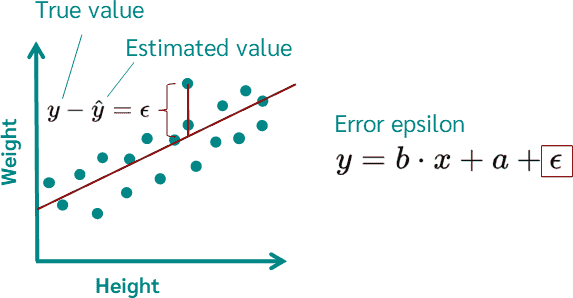
The linear regression model is

$$y_i = \mathbf{x}_i^T\boldsymbol{\beta} + \varepsilon_i.$$

For a single predictor $x_i$, this becomes

$$y_i = \beta_0 + \beta_1x_i + \varepsilon_i,$$

where $\beta_0$ is the intercept and $\beta_1$ is the slope.

Stacking all observations produces the matrix form

$$\mathbf{y} = \mathbf{X}\boldsymbol{\beta} + \boldsymbol{\varepsilon},$$

with

$$\mathbf{y} \in \mathbb{R}^{n}, \qquad \mathbf{X} \in \mathbb{R}^{n\times(p+1)}, \qquad \boldsymbol{\beta} \in \mathbb{R}^{p+1}.$$

The model is linear in its parameters. The predictors themselves need not appear only as raw values. Polynomial terms, interactions, logarithms, and other transformations may be included as columns of $\mathbf{X}$ while the model remains a linear regression model. For example,

$$y_i = \beta_0 + \beta_1x_i + \beta_2x_i^2 + \varepsilon_i$$

is linear in $\beta_0$, $\beta_1$, and $\beta_2$, even though it is nonlinear in $x_i$.

Ordinary least squares

For a candidate coefficient vector $\boldsymbol{\beta}$, the fitted values and residuals are

$$\hat{\mathbf{y}} = \mathbf{X}\boldsymbol{\beta}, \qquad \mathbf{e} = \mathbf{y} - \hat{\mathbf{y}}.$$

Ordinary least squares (OLS) selects the coefficients that minimize the residual sum of squares:

$$\hat{\boldsymbol{\beta}}_{\mathrm{OLS}} = \underset{\boldsymbol{\beta}}{\operatorname{arg\,min}} \left\| \mathbf{y}-\mathbf{X}\boldsymbol{\beta} \right\|_2^2.$$

Equivalently, the objective is

$$S(\boldsymbol{\beta}) = (\mathbf{y}-\mathbf{X}\boldsymbol{\beta})^T (\mathbf{y}-\mathbf{X}\boldsymbol{\beta}).$$

Expanding the quadratic expression gives

$$S(\boldsymbol{\beta}) = \mathbf{y}^T\mathbf{y} -2\boldsymbol{\beta}^T\mathbf{X}^T\mathbf{y} +\boldsymbol{\beta}^T\mathbf{X}^T\mathbf{X}\boldsymbol{\beta}.$$

Differentiating with respect to $\boldsymbol{\beta}$ yields

$$\nabla_{\boldsymbol{\beta}}S = -2\mathbf{X}^T\mathbf{y} +2\mathbf{X}^T\mathbf{X}\boldsymbol{\beta}.$$

Setting the gradient to zero produces the normal equations:

$$\mathbf{X}^T\mathbf{X}\hat{\boldsymbol{\beta}} = \mathbf{X}^T\mathbf{y}.$$

If $\mathbf{X}$ has full column rank, then $\mathbf{X}^T\mathbf{X}$ is invertible and the solution is unique:

$$\boxed{ \hat{\boldsymbol{\beta}}_{\mathrm{OLS}} = (\mathbf{X}^T\mathbf{X})^{-1}\mathbf{X}^T\mathbf{y} }.$$

This closed-form expression is valuable for analysis. In numerical software, however, explicitly computing the inverse is generally discouraged because it is less stable and less efficient than solving the least-squares system with QR decomposition or singular value decomposition (SVD).

Geometric interpretation

The vector of fitted values is

$$\hat{\mathbf{y}} = \mathbf{X}\hat{\boldsymbol{\beta}} = \mathbf{H}\mathbf{y},$$

where

$$\mathbf{H} = \mathbf{X}(\mathbf{X}^T\mathbf{X})^{-1}\mathbf{X}^T$$

is the hat matrix.

OLS projects $\mathbf{y}$ onto the column space of $\mathbf{X}$. At the optimum, the residual vector is orthogonal to every column of the design matrix:

$$\mathbf{X}^T\mathbf{e} = \mathbf{0}.$$

This orthogonality condition is another form of the normal equations. When the model includes an intercept, it also implies that the residuals sum to zero.

Maximum likelihood estimation

OLS defines an optimization criterion without requiring a complete probability distribution for the errors. Maximum likelihood estimation (MLE), by contrast, begins with a probabilistic model.

Assume that the errors are independent and normally distributed with constant variance:

$$\varepsilon_i \overset{\mathrm{i.i.d.}}{\sim} \mathcal{N}(0,\sigma^2).$$

It follows that

$$y_i\mid\mathbf{x}_i \sim \mathcal{N}(\mathbf{x}_i^T\boldsymbol{\beta},\sigma^2)$$

and, in matrix form,

$$\mathbf{y}\mid\mathbf{X} \sim \mathcal{N}(\mathbf{X}\boldsymbol{\beta},\sigma^2\mathbf{I}).$$

The likelihood is

$$p(\mathbf{y}\mid\mathbf{X},\boldsymbol{\beta},\sigma^2) = (2\pi\sigma^2)^{-n/2} \exp\left[ -\frac{1}{2\sigma^2} (\mathbf{y}-\mathbf{X}\boldsymbol{\beta})^T (\mathbf{y}-\mathbf{X}\boldsymbol{\beta}) \right].$$

Taking the logarithm gives

$$\ell(\boldsymbol{\beta},\sigma^2) = -\frac{n}{2}\log(2\pi) -\frac{n}{2}\log(\sigma^2) -\frac{1}{2\sigma^2} \left\| \mathbf{y}-\mathbf{X}\boldsymbol{\beta} \right\|_2^2.$$

For fixed $\sigma^2$, the first two terms do not depend on $\boldsymbol{\beta}$. Maximizing the log-likelihood is therefore equivalent to minimizing the residual sum of squares:

$$\hat{\boldsymbol{\beta}}_{\mathrm{MLE}} = \hat{\boldsymbol{\beta}}_{\mathrm{OLS}}.$$

Thus, OLS and MLE produce the same coefficient estimate under independent Gaussian errors with constant variance. They arrive there from different starting points: OLS minimizes a geometric loss, whereas MLE maximizes the probability assigned to the observed data.

Estimating the error variance

Substituting $\hat{\boldsymbol{\beta}}$ into the likelihood and optimizing with respect to $\sigma^2$ gives

$$\hat{\sigma}_{\mathrm{MLE}}^2 = \frac{1}{n} \left\| \mathbf{y}-\mathbf{X}\hat{\boldsymbol{\beta}} \right\|_2^2.$$

This is the maximum likelihood estimator, but it is biased downward because the same data were used to estimate the regression coefficients. Under the classical model, the commonly used unbiased estimator is

$$s^2 = \frac{1}{n-p-1} \left\| \mathbf{y}-\mathbf{X}\hat{\boldsymbol{\beta}} \right\|_2^2.$$

The denominator $n-p-1$ represents the residual degrees of freedom when the model contains $p$ predictors and one intercept.

Assumptions and their consequences

It is useful to distinguish assumptions needed to estimate coefficients from assumptions needed for optimality and statistical inference.

Linearity of the conditional mean

The model assumes

$$\mathbb{E}[\mathbf{y}\mid\mathbf{X}] = \mathbf{X}\boldsymbol{\beta}.$$

This does not require every observed point to lie near a straight line. It requires the expected response, conditional on the selected features and transformations, to have the specified linear form.

Exogeneity

The error must have conditional mean zero:

$$\mathbb{E}[\boldsymbol{\varepsilon}\mid\mathbf{X}] = \mathbf{0}.$$

This assumption fails when relevant variables are omitted and correlated with included predictors, when predictors are measured with error, or when the response influences a predictor. Under such conditions, an estimated coefficient should not be interpreted causally without an appropriate research design.

Full column rank

No predictor column may be an exact linear combination of the others. Exact multicollinearity prevents a unique OLS solution. Strong but imperfect multicollinearity does not prevent estimation, but it increases coefficient uncertainty and makes individual estimates sensitive to small changes in the data.

Homoscedasticity and uncorrelated errors

The classical model assumes

$$\operatorname{Var}(\boldsymbol{\varepsilon}\mid\mathbf{X}) = \sigma^2\mathbf{I}.$$

Under linearity, exogeneity, full rank, and this covariance assumption, the Gauss–Markov theorem states that OLS is the best linear unbiased estimator: among linear unbiased estimators, it has the smallest variance.

Heteroscedasticity or correlated errors do not automatically bias the OLS coefficients when exogeneity still holds. They do, however, invalidate the usual standard errors and reduce efficiency. Heteroscedasticity-consistent or cluster-robust covariance estimators may be required.

Normality

Normally distributed errors are not required to compute OLS estimates or for the Gauss–Markov result. Normality provides the exact finite-sample distributions used for classical $t$ tests, $F$ tests, and confidence intervals. In sufficiently large samples, asymptotic inference may remain useful without exact normality, subject to the other assumptions and appropriate standard errors.

Interpreting coefficients

In a multiple regression model,

$$\mathbb{E}[y\mid\mathbf{x}] = \beta_0+\beta_1x_1+\cdots+\beta_px_p,$$

$\beta_j$ is the expected change in the response associated with a one-unit increase in $x_j$, holding the other included predictors constant.

This interpretation requires care:

• The unit of measurement determines the numerical scale of a coefficient.
• A coefficient describes association unless the study design supports a causal claim.
• Interaction terms make a predictor’s effect depend on another predictor.
• Polynomial terms make the marginal effect vary with the predictor value.
• Extrapolation beyond the observed feature range can be unreliable even when the fitted line appears reasonable.

For example, if

$$\widehat{\mathrm{price}} = 50{,}000 +180\,(\mathrm{area}) -8{,}000\,(\mathrm{age}),$$

then, within the model and observed data range, one additional unit of area is associated with an expected price increase of $180$, holding age constant. The coefficient alone does not establish that increasing area would cause exactly that change in every case.

Statistical uncertainty

Under the classical homoscedastic model,

$$\operatorname{Var}(\hat{\boldsymbol{\beta}}\mid\mathbf{X}) = \sigma^2(\mathbf{X}^T\mathbf{X})^{-1}.$$

Replacing $\sigma^2$ with $s^2$ yields estimated standard errors. These quantify sampling uncertainty in the coefficients and form the basis of confidence intervals and hypothesis tests.

A confidence interval for a mean response is narrower than a prediction interval for a new observation. The latter must account for both uncertainty in the estimated mean and the irreducible observation error.

Statistical significance should not be treated as practical significance. A small effect can have a very small $p$-value in a large dataset, while an operationally important effect may remain uncertain in a small dataset. Coefficient magnitude, uncertainty, units, and domain context should be reported together.

Model evaluation

For observed responses $y_i$, fitted values $\hat{y}_i$, and mean response $\bar{y}$, common metrics include:

Mean squared error

$$\operatorname{MSE} = \frac{1}{n}\sum_{i=1}^{n}(y_i-\hat{y}_i)^2.$$

MSE strongly penalizes large errors and uses squared response units.

Root mean squared error

$$\operatorname{RMSE} = \sqrt{\operatorname{MSE}}.$$

RMSE is expressed in the same units as the response, which often makes it easier to interpret.

Coefficient of determination

$$R^2 = 1- \frac{\sum_{i=1}^{n}(y_i-\hat{y}_i)^2} {\sum_{i=1}^{n}(y_i-\bar{y})^2}.$$

$R^2$ measures the proportion of sample variation explained relative to an intercept-only model. It does not measure causal validity, guarantee good out-of-sample prediction, or confirm that the model assumptions hold. Adding predictors cannot decrease the training $R^2$, so adjusted $R^2$ or out-of-sample evaluation is more informative when comparing models of different sizes.

Predictive performance should be measured on validation or test data that were not used to estimate the coefficients. For time-dependent or grouped observations, the data split must preserve the relevant dependence structure.

Residual diagnostics

Residual analysis tests whether the fitted model is compatible with its assumptions.

• Residuals versus fitted values: curvature suggests a missing nonlinear term; a funnel shape suggests non-constant variance.
• Quantile–quantile plot: substantial deviations from a straight reference line indicate non-normal tails or outliers.
• Residuals versus time or sequence: systematic patterns suggest autocorrelation.
• Leverage and influence: observations with unusual predictor values can have a disproportionate effect on the fitted coefficients.
• Variance inflation factors: large values can reveal unstable estimation caused by multicollinearity.

Diagnostics should inform model revision, not serve as a mechanical pass-or-fail checklist. A visible pattern may indicate a missing transformation, interaction, group effect, nonlinear model, or different error structure.

Regularized linear regression

When the feature set is large or predictors are strongly correlated, regularization can improve out-of-sample performance.

Ridge regression

Ridge regression adds an $L_2$ penalty:

$$\hat{\boldsymbol{\beta}}_{\mathrm{ridge}} = \underset{\boldsymbol{\beta}}{\operatorname{arg\,min}} \left\{ \left\|\mathbf{y}-\mathbf{X}\boldsymbol{\beta}\right\|_2^2 +\lambda\sum_{j=1}^{p}\beta_j^2 \right\}.$$

It shrinks coefficients toward zero and stabilizes estimates under multicollinearity.

Lasso regression

Lasso uses an $L_1$ penalty:

$$\hat{\boldsymbol{\beta}}_{\mathrm{lasso}} = \underset{\boldsymbol{\beta}}{\operatorname{arg\,min}} \left\{ \left\|\mathbf{y}-\mathbf{X}\boldsymbol{\beta}\right\|_2^2 +\lambda\sum_{j=1}^{p}|\beta_j| \right\}.$$

The $L_1$ penalty can set some coefficients exactly to zero, producing a sparse model. The regularization strength $\lambda$ should be selected using validation data or cross-validation. Predictors are usually standardized before penalization, and the intercept is normally excluded from the penalty.

A numerically stable implementation

The analytical formula contains $(\mathbf{X}^T\mathbf{X})^{-1}$, but production code should solve the least-squares problem directly:

import numpy as np


def fit_linear_regression(features, targets):
    """Return OLS coefficients, including an intercept."""
    x = np.asarray(features, dtype=float)
    y = np.asarray(targets, dtype=float)

    design = np.column_stack([np.ones(x.shape[0]), x])
    coefficients, _, rank, singular_values = np.linalg.lstsq(
        design,
        y,
        rcond=None,
    )

    if rank < design.shape[1]:
        raise ValueError("The design matrix is rank deficient.")

    return coefficients, singular_values

numpy.linalg.lstsq uses a numerically appropriate factorization and also exposes information about rank and singular values. A complete analysis should additionally retain residuals, estimate uncertainty, examine diagnostics, and evaluate predictions on unseen data.

Conclusion

Linear regression combines a clear mathematical structure with broad practical utility:

• OLS estimates coefficients by minimizing the sum of squared residuals.
• Under independent Gaussian errors with constant variance, the OLS coefficient estimate is also the maximum likelihood estimate.
• Normality is required for exact classical inference, not for computing the OLS solution.
• Coefficients describe conditional associations and require additional assumptions for causal interpretation.
• Residual diagnostics and out-of-sample evaluation are essential; a high training $R^2$ is not sufficient evidence of a reliable model.
• QR- or SVD-based least-squares solvers are preferable to explicitly inverting $\mathbf{X}^T\mathbf{X}$.

Linear regression is therefore more than a formula for fitting a line. It is a compact framework for understanding estimation, uncertainty, assumptions, and the distinction between fitting observed data and building a model that generalizes.